LAB 3: INTENSITY TRANSFORMATION (MATLAB)

assalamualaikum to our fellow lecturer and friends. have you ever heard about intensity transformation and spatial filtering? this week, we have learned something new about matlab which are intensity transformation and spatial filtering. there are four main function of intensity transformation:

• photographic negative (using imcomplement)
• gamma transformation (using imadjust)
• logaritmic transformation (using c*log(1+f))
• contrast-stretching transformations (using 1./(1+(m./(double(f)+eps)).^E)

photographic negative (using imcomplement) 

then what is photographic negative? ok, in the easiest words, it means that the true black becomes true white and vise versa. matlab has a function to create this photographic negative by imcomplement (f). lets see our coding example that we have done during lab session :)

>>   I=imread('cat.JPG')

>>  J=imcomplement(I);

>>  imshow(I)

>>  figure, imshow(J)

original image

after photographic negative

gamma tranformation (using imadjust)

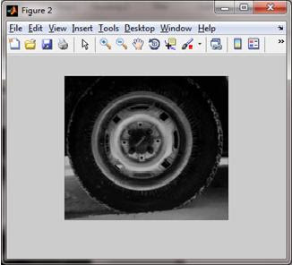
next is about gamma transformations. what is gamma transformation? with gamma transformation, we can curve the grayscale components either to brighten the intensity or to darken the instensity. when the component grayscale darken, it means the gamma is less than one and vice versa. lets see the coding example of gamma transformation :)

>>   I = imread('tire.tif');

>>   J=imadjust(I,[],[],1);

>>   J2=imadjust(I,[],[],3);

>>   J3=imadjust(I,[],[],0.4);

>>   imshow(J);

>>   figure, imshow (J2);

>>   figure, imshow (J3);

J

J2

J3

logaritmic transformations (using c*log(1+f))

usually, logarithmic transformation used to brighten the intensities of an image of lower intensity values. its function in matlab can be shown as,    g = c*log(1+double(f)) . here, we paste some matlab code example  for logaritmic transformation :)

>>   I = imread('tire.tif');

>>   I2=im2double(I);

>>   J=1*log(1+I2);

>>   J2=2*log(1+I2); 

>>   J3=5*log(1+I2); 

>>   imshow(I) 

>>   figure, imshow(J)

>>   figure, imshow(J2)

>>   figure, imshow(J3)

original image

J

J2

J3

contrast-stretching transformations (using 1./(1+(m./(double(f)+eps)).^E) 

this is the last part of intensity transformation for our lab. what is contrast-stretching transformation? urm, contrast-stretching transformation results in increasing the contrast between the darks and the lights. this will end up the dark being darker and the lights being lighter, with only few levels of gray in between. lets see our coding example and screenshot in plot form to enable readers to make contrast comparison easily :)

a)  light to lighter

>> I = imread('tire.tif');

>> I2=im2double(I);

>> m=mean2(I2)

>> contrast1=1./(1+(m./(I2+eps)).^4);

>> contrast2=1./(1+(m./(I2+eps)).^5);

>> contrast3=1./(1+(m./(I2+eps)).^10);

>> figure(1), subplot(2,2,1),imshow(I2),xlabel('I2')

>> figure(1), subplot(2,2,2),imshow(contrast1),xlabel('contrast 1')

>> figure(1), subplot(2,2,3),imshow(contrast2),xlabel('contrast 2')

>> figure(1), subplot(2,2,4),imshow(contrast3),xlabel('contrast 3')

(a) contrast-stretching transformation. bright to brighter. 

a)  dark to darker

>> I = imread ('tire.tif');

>> I2=im2double(I);

>> contrast1 = 1./(1+(0.2./(I2+eps)).^4);

>> contrast2 = 1./(1+(0.5./(I2+eps)).^4);

>> contrast3 = 1./(1+(0.7./(I2+eps)).^4);

>>figure(1), subplot(2,2,1), imshow(I2), xlabel('I2')

>>figure(1), subplot(2,2,2), imshow(contrast1), xlabel('contrast1')

>>figure(1), subplot(2,2,3), imshow(contrast2), xlabel('contrast2')

>>figure(1), subplot(2,2,4), imshow(contrast3), xlabel('contrast3')

(b) contrast-stretching transformation. dark to darker. 

we hope our post on this time will help you to understand a little bit about intensity transformation. in the next post, we will update about the spatial filtering in matlab. thanks you :)